OOMMF Tutorial Part 4: OOMMF Analysis Tools
When doing micromagnetic simulations it is easy to end up with hundreds of output files, so part four of this OOMMF Tutorial covers some of the tools available for analysing OOMMF data. This list isn’t exhaustive - if I’ve missed out your favourite - please leave a comment! OOMMF outputs two types of data: vector, such as magnetisation or demagnetising fields; and scalar such as energies and total magnetisations. There are tools available for processing both types. If you haven’t already please check out parts one, two and three of this tutorial.
Built-in analysis tools
OOMMF already comes with some simple tools for viewing, saving and analysing your data. They’re not necessarily the most advanced, or easy to use, but they allow at least for quickly checking progress of calculations so can be invaluable.
mmDisp
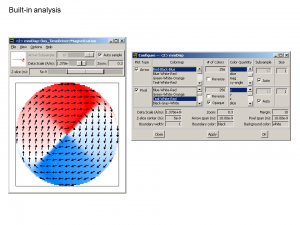
The most straight forward tool for analysing vector data is to use mmDisp. You can even set OOMMF to automatically display to mmDisp as the calculation runs.
 |
|---|
| Using mmDisp to examine magnetisation vector data. |
With mmDisp you can view different components of vector data as well as derivatives. You can select from a number of different colour schemes for both image pixels and arrows. See more about mmDisp in the OOMMF documentation.
mmGraph
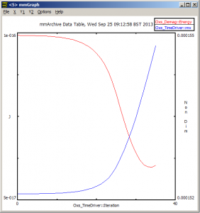
mmGraph is the scalar equivalent of mmDisp. It lets you quickly and easily view the data table output from your OOMMF simulations. In terms of functionality the plotter is quite straightward, so you’ll probably want to use separate software for producing production quality graphs.
 |
|---|
| Built-in graph viewer. Plot different scalar parameters such as simulation time, total energy, magnetisation. |
You can export the plotted data as a graphic, but I often cheat by using Alt+Print Screen to copy the window to the clip board. I find this handy for quickly producing summaries of simulations. See more about mmGraph in the OOMMF documentation.
External Tools
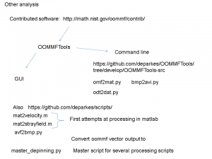
There are a number of different external tools for analysing oommf data. Many of them are listed on the oommf nist website (link). I will focus on OOMMFTools since that is the one that I am most familiar with.
OOMMFTools
OOMMFTools is a suite of tools designed to make it easier to analyse OOMMF output data. The tools come in GUI and a command line form. The suite of tools makes it easy to convert single or multiple OOMMF files into other formats more readily viewed or further processed than the standard output formats.
 |
|---|
| Options for processing oommf data with oommf tools. |
The basic operations available in OOMMFTools are vector format -> matlab/python readable file; vector format -> bitmap, video; scalar data table -> plain text.
odt2dat.py
To make the scalar data table easier to understand it is good to convert it to a plain text ascii .dat file. odt2dat.py lets you do this. The column headings are shown below. Once you know the number of the column you can easily plot it against any other column using your favourite graphing software.
1
2
3
4
5
6
7
8
9
10
11
12
13
14
15
16
17
18
19
20
21
22
23
24
Total energy
Energy calc count
Max dm/dt
dE/dt
Delta E
FeGa UniformExchange Energy
Max Spin Ang
Stage Max Spin Ang
Run Max Spin Ang
Strain Energy
UZeeman Energy
B
Bx
By
Bz
Demag Energy
Iteration
Stage iteration
Stage
mx
my
mz
Last time step
Simulation time
omf2mat.py
Easily convert vector outputs into matlab .mat files or python pickle files. From there it is easy to extract line scans and perform more advanced analysis on individual cells in the mesh. I’ll show a sample matlab m file to read in the resulting .mat file in a future post.
avf2bmp.py
This is essentially a wrapper for the built-in OOMMF command line program avf2ppm.py. It uses your OOMMF install to convert vector files to bitmaps.
1
avf2bmp.py my_omf.omf
for single files, or run
1
avf2bmp.py *.omf
for all .omf files in the directory.
bmp2avi.py
One of the most striking ways to present time-evolving data is as a video. OOMMFTools uses ffmpeg (available as part of ImageMagick) to convert a folder of bitmaps into an avi video.
You might also consider
There are some other tools that I’m not so familiar with that you might also be interested in using. The best place to find analysis tools is probably the OOMMF website.