Monte Carlo Simulation
Monto Carlo simulation is a technique for approximating future behaviour based on randomly sampled numbers. By sampling from different probability distributions it is possible to use Monte Carlo simulation for a range of different situations including physical systems, computer games or finance. This post gives a simple example of Monte Carlo simulation to give some of the essential background features. Monte Carlo simulation is related to the similar concept of Monte Carlo integration.
Monte Carlo Simulation
I’ve tried to come up with an example of where you could use Monte Carlo Simulation to help decision making. Imagine you work in a post office and want to know if three desks is enough to keep the queue from going above 20 people.
You spend a day watching customers arrive and staff go about their work. You find that customers arrive at a rate of 0.9 per minute and that in a given minute there is a 50 per cent chance that a busy desk will clear.
To build a model we can use a Poisson distribution for the arrivals, with a lambda value of 0.9 (the mean number of occurrences in the one minute time interval). We can simulation the behaviour of a desk clearing or not using a uniform distribution, taking it to be cleared if the probability is greater than 0.7. Using this information we can create a simple Monte Carlo simulation.
Single Run
We begin with a single run of the simulation. We play forward time for 300 minutes to see what happens. Here’s an implementation of such a simulation in python:
1
2
3
4
5
6
7
8
9
10
11
12
13
14
15
16
17
18
19
20
%matplotlib inline
from scipy import random
import numpy as np
import matplotlib.pyplot as plt
number_of_desks = 3
number_of_minutes = 300
queue = 0
queue_size_over_time = [queue]
for i in range(number_of_minutes):
    arrivals_in_a_minute = random.poisson(lam=0.9)
    jobs_processed_in_a_minute = sum(random.uniform(size=number_of_desks) > 0.7)
    # Number of arrivals get added to a queue
    queue += (arrivals_in_a_minute - jobs_processed_in_a_minute)
    if queue < 0:
        queue = 0
    queue_size_over_time.append(queue)
plt.plot(queue_size_over_time)
plt.xlabel('Number of Minutes')
plt.ylabel('Queue Size')
plt.show()
For a single run of this code it suggests that the queue grows to a size of around 25 and stays there.:
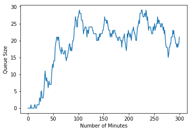 |
|---|
| monte carlo simulation single run example |
Of course that was just a single run of randomly selected possibilities. If we run the simulation again we get a different result, which suggests a peak
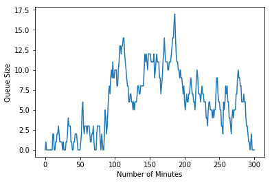 |
|---|
| monte carlo simulation second run |
Which simulation should we believe? This is the random element of the Monte Carlo simulation at play - for us to use our simulation to help us make a decision we should make many more runs of the simulation. Rather than doing this manually, we can modify the script to repeat it many times for us.
Multiple Runs
Running multiple times is where this simple Monte Carlo simulation really contributes. We can modify the simulation code to run 1000 times instead of just once, and also capture some basic statistics of mean and maximum run times for each run.
1
2
3
4
5
6
7
8
9
10
11
12
13
14
15
16
17
18
19
20
21
22
23
24
25
26
27
28
29
30
31
32
33
34
%matplotlib inline
from scipy import random
import numpy as np
import matplotlib.pyplot as plt
number_of_desks = 3
number_of_minutes = 300
number_of_test_runs = 1000
mean_queue_size = []
max_queue_size = []
for i in range(number_of_test_runs):
    queue = 0
    queue_size_over_time = [queue]
    for i in range(number_of_minutes):
        arrivals_in_a_minute = random.poisson(lam=0.9)
        jobs_processed_in_a_minute = sum(random.uniform(size=number_of_desks) > 0.7)
        # Number of arrivals get added to a queue
        queue += (arrivals_in_a_minute - jobs_processed_in_a_minute)
        if queue < 0:
            queue = 0
        queue_size_over_time.append(queue)
    mean_queue_size.append(np.mean(queue_size_over_time))
    max_queue_size.append(np.max(queue_size_over_time))
    plt.plot(queue_size_over_time)
plt.xlabel('Number of Minutes')
plt.ylabel('Queue Size')
plt.show()
plt.hist(mean_queue_size, ec='black')
plt.xlabel('Mean Queue Size')
plt.ylabel('Count')
plt.show()
plt.hist(max_queue_size, ec='black')
plt.xlabel('Max. Queue Size')
plt.ylabel('Count')
plt.show()
The graph of queue size over time is predictably dense:
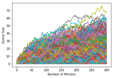 |
|---|
| monte carlo simulation - multiple time graphs |
From this rather chaotic mess we can extract some insight using the statistics we gathered. Histograms of the mean
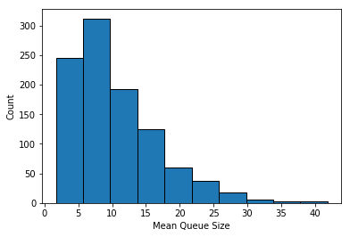 |
|---|
| monte carlo simulation - mean queue size |
and maximum queue lengths
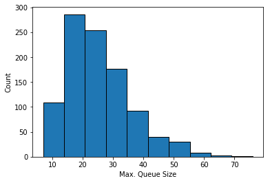 |
|---|
| monte carlo simulation - max queue size |
of each simulation suggest that 3 desks is not enough to keep queue lengths to an acceptable level.
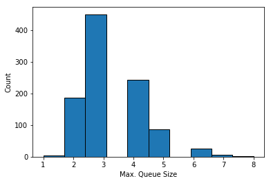
Experimenting with Monte Carlo Simulations
Having concluded that our initial suggestion of three desks in the post office isn’t enough, we can use Monte Carlo simulation to estimate how many desks would be needed. As a single comparison I’ve re-run the 1000 simulations with 10 desks instead of 3. Looking at the histogram of maximum queue sizes suggests that this would be enough to keep the queue size low enough:
 |
|---|
| monte carlo simulation - max queue size with 10 desks |