Monte Carlo Integration
Monte Carlo integration uses random numbers to approximate the solutions to integrals. While not as sophisticated as some other numerical integration techniques, Monte Carlo integration is still a valuable tool to have in your toolbox.
Monte Carlo integration is one type of Monte Carlo method - a family of techniques which use randomly generated numbers to estimate or simulate different problems.
Monte Carlo Integration
The basic idea is that an integral can be approximated as (taking a 2d example - Wikipedia has a more general example):
\[I=\int^b_af(x)dx\]The result of the integral can be approximated as:
\[I\approx\dfrac{a-b}{N}\sum_{i}^{N}f(x_i)\]where N is the number of random numbers and a and b are lower and upper bounds of the integral respectively. It is in this approximation that the Monte Carlo aspect comes in: we generate a large number of random numbers to get an approximation for the value of the integral.
This video has a good description of this approximation as well as an example implementation in python.
An Example in Python
We can construct a simple example in python First the setup: we want to integrate the simple function y = 3x between 1 and 10. We can either work this out ourselves or use Wolfram alpha. Either way, the analytical solution in 148.5 First we import the necessary modules.
1
2
3
4
%matplotlib inline # useful if you are using jupyter notebooks
from scipy import random
import numpy as np
import matplotlib.pyplot as plt
Then we set up the limits of the integral and the function we wish to integrate. Here I’ve got a simple example, but in general you could have any arbitrary function of x.
1
2
3
4
lower = 1
upper = 10
def function_to_integrate(x):
    return 3*x
Now we can get into the Monte Carlo integration part. For this we will need a large number, N, of uniformly distributed random numbers within the limits of the integral.
1
2
N = 1000
random_numbers = random.uniform(lower, upper, N)
Then, to actually run the Monte Carlo integration we can simply loop through each of the random numbers, keeping a running total of the estimated integral as we go.
1
2
3
estimated_integral = 0.0
for random_number in random_numbers:
    estimated_integral += function_to_integrate(random_number)
The final stage is to multiply by the coefficient determined by the limits of the integral and the number of random numbers used.
1
2
estimate = (upper-lower)/float(N)*estimated_integral
print("A single estimate for the integral of the function is: ", estimate)
The first time I ran it I got an answer of 151.3. Not bad.
Multiple Estimates
Having written the code to make one estimate using Monte Carlo integration, it is not too much more work to make multiple estimates. We just need to keep track of each estimate we make.
This is similar to the concept of boot strapping and other resampling methods. To do this we put the original Monte Carlo integration estimator in a function and call it multiple times, M. Each estimate gets appended to a list so we can calculate the mean value at the end.
1
2
3
4
5
6
7
8
9
10
11
12
13
14
15
16
17
18
19
20
21
%matplotlib inline
from scipy import random
import numpy as np
import matplotlib.pyplot as plt
lower = 1
upper = 10
N = 1000
def function_to_integrate(x):
    return 3*x
def single_estimate():
    estimated_integral = 0.0
    random_numbers = random.uniform(lower, upper, N)
    for random_number in random_numbers:
        estimated_integral += function_to_integrate(random_number)
    return (upper-lower)/float(N)*estimated_integral
print("A single estimate for the integral of the function is: ", single_estimate())
M = 100
multiple_estimates = []
for n in range(M):
    multiple_estimates.append(single_estimate())
print("The average of all estimates was: ", np.mean(multiple_estimates))
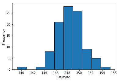
Which gave an average of all the estimates of 148.4, which is rather close to the analytically derived value. Taking multiple estimates also means we can calculate a standard deviation with np.std(multiple_estimates). I got the value of 2.3.
Having the mean and standard deviation of your Monte Carlo Integration estimates means you can also think about calculating confidence intervals for the estimate. We can visualise the different estimates as a histogram. The distribution is centered on the true value of 148.5.
1
2
3
plt.hist(multiple_estimates, bins=10, ec='black')
plt.ylabel('Frequency')
plt.xlabel('Estimate')
 |
|---|
| Example Histogram |
Try playing with different values for N (the number of random numbers per estimate), and M (the number of estimates) and see what you get. Also see what values you get for mean (use np.mean(multiple_estimates) and standard deviation