OOMMF Tutorial Part 7: Field Pulses
In part 7 of this OOMMF tutorial I will show you how to excite a simulation with a field pulse in OOMMF.
Defining The Field Pulse
Using Oxs_ScriptUZeeman we can define our field pulse as more or less any function, but in this tutorial We’ll be trying to make this pulse made up of a rising and falling exponential:
 |
|---|
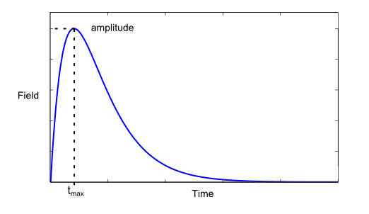
| OOMMF Field Pulse |
Oxs_ScriptUZeeman will require the function and its derivative with respect to time. We’ll define separately the rising and falling exponentials that define the field pulse:
rising exponential: \(f_1 = 1-exp(-\frac{t}{a})\); derivative: \(df_1 = \frac{exp(-\frac{t}{a})}{a}\) falling exponential: \(f_2 = exp(-\frac{t-b}{a})\); derivative: \(df_2 = -\frac{exp(-\frac{t-b}{c})}{c}\)
We will later multiply the two exponentials together, and determining the derivative of the resulting function using the chain rule. By equating the differential to zero we can find the time which gives maximum field:
\[t_{max}=alog(-\frac{(-a-c)}{a})]\]which gives a corresponding maximum field of
\[(1-exp(-\frac{t_{max}}{a}))exp(-\frac{t_{max}-b}{a})\]We will be using the Oxs_ScriptUZeeman which takes this form:
Specify Oxs_ScriptUZeeman:name {
  script_args { args_request }
  script Tcl_script
  multiplier multiplier
  stage_count number_of_stages
}
Combined with a tcl procedure to define the pulse profile:
#  Set the field pulse proc
#  Pass to it the different constants making up the exponentials
proc FieldPulse { Amp a b c stage stage_time total_time  } {
   set rise   [expr {(1-exp(-$total_time/($a)))}]
   set fall   [expr {exp(-($total_time-($b))/($a))}]
   set drise  [expr {exp(-$total_time/($a))/($a)}]
   set dfall  [expr {-exp(-($total_time-($b))/($c))/$c}]
   set tmax [expr {$a*log(-(-$a-$c)/$a)}]
   set Hmax [expr {(1-exp(-$tmax/($a)))*exp(-($tmax-($b))/($a))}]
   set A [expr {$Amp/$Hmax}]
   set Hy   [expr {$A*$rise*$fall}]
   set dHy  [expr {$A*($rise*$dfall+$drise*$fall)}]
   return [list $Hy 0 0 $dHy 0 0]
}
Those are the basic building blocks needed to include a field pulse in an oommf simulation, but it would be instructive to look an example.
An example:
As an example, let’s modify the example square.mif (found in /oommf/app/oxs/examples/) You can download the modified file here.
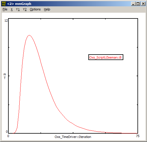
mmGraph output
When we run square_fieldpulse.mif we can see the applied field pulse in mmGraph, as shown below.
 |
|---|
| More Field Functions |
You can easily modify this basic field pulse recipe for your own functions. Just define the function, find its derivative and put it into the ‘FieldPulse’ procedure. For help plotting the functions and finding the derivative you might want to use Wolfram Alpha.