A few ways to do linear regressions on data in python. Linear regression is a simple and common technique for modelling the relationship between dependent and independent variables. This post gives you a few examples of Python linear regression libraries to help you analyse your data. Which method is best for you will probably depend on exactly what you are doing. The scipy method is a bit more ‘bare-bones’; the statsmodels method is part of an extensive “traditional” statistics module; while the sklearn approach would probably be best if you are working on a larger machine learning project.
Method 1: Scipy
Scipy is a python analysis ecosystem that encapsulates a few different libraries such as numpy and matplotlib. Here I’ve picked out two approaches you could use: linregress and polyfit
With linregress
Firstly I’ll use the ‘linregress’ linear regression function.
1
2
3
4
5
6
7
8
| # load iris sample dataset
import seaborn.apionly as sns
iris = sns.load_dataset('iris')
# import scipy
from scipy import polyval, stats
fit_output = stats.linregress(iris["petal_length"], iris["petal_width"])
slope, intercept, r_value, p_value, slope_std_error = fit_output
print(slope, intercept)
|
To estimate y-values using these fitting parameters we can use the scipy/numpy ‘polyval’ function:
1
2
3
| # use scipy polyval to create y-values from x_data and the
# linregress fit parameters
scipy_fitted_y_vals = polyval([slope,intercept],iris["petal_length"])
|
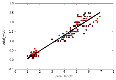
Which we can plot along with the original data
1
2
3
4
| import matplotlib.pyplot as plt
axes = iris.plot(x="petal_length", y="petal_width", kind="scatter", color="red")
plt.plot(iris["petal_length"], scipy_fitted_y_vals, color='black', linewidth=3)
plt.show()
|
|
|---|
| python linear regression - linregress |
With polyfit
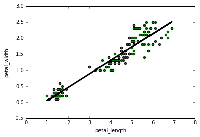
While still using scipy, you can also use the polyfit function. As its name suggests it can be used to fit higher order polynomials, but here we’ll just use it for a linear regression:
1
2
3
4
5
6
7
8
| form scipy import polyfit
# fit with scipy polyfit
(slope, intercept) = polyfit(iris["petal_length"], iris["petal_width"], 1)
scipy_fitted_y2 = polyval([slope, intercept], iris["petal_length"])
import matplotlib.pyplot as plt
axes = iris.plot(x="petal_length", y="petal_width", kind="scatter", color="green")
plt.plot(iris["petal_length"], scipy_fitted_y2, color='black', linewidth=3)
plt.show()
|
|
|---|
| python linear regression - polyfit |
Method 2: statsmodels
statsmodels is a python module dedicated to statistcal modelling and testing. statsmodels has many advanced fitting and regression libraries, as well as simpler ones like linear regression. One important way that statsmodels differs from other regression modules is that it doesn’t automatically add a constant intercept to the regression - we need to do that ourselves.
1
2
3
4
5
6
7
8
9
10
| # load iris sample dataset
import seaborn.apionly as sns
iris = sns.load_dataset('iris')
import statsmodels.api as sm
# fit with statsmodels
# add constant intercept
X = sm.add_constant(iris["petal_length"])
model = sm.OLS(iris["petal_length"], X)
results = model.fit()
statsmodels_y_fitted = results.predict()
|
With statsmodels you can also print out a comprehensive report on fit:
1
| print(results.summary())
|
which gives this output
1
2
3
4
5
6
7
8
9
10
11
12
13
14
15
16
17
18
19
20
21
22
| OLS Regression Results
==============================================================================
Dep. Variable: y R-squared: 0.927
Model: OLS Adj. R-squared: 0.927
Method: Least Squares F-statistic: 1882.
Date: Sat, 12 Nov 2016 Prob (F-statistic): 4.68e-86
Time: 11:08:10 Log-Likelihood: 24.796
No. Observations: 150 AIC: -45.59
Df Residuals: 148 BIC: -39.57
Df Model: 1
Covariance Type: nonrobust
================================================================================
coef std err t P>|t| [95.0% Conf. Int.]
--------------------------------------------------------------------------------
const -0.3631 0.040 -9.131 0.000 -0.442 -0.285
petal_length 0.4158 0.010 43.387 0.000 0.397 0.435
==============================================================================
Omnibus: 5.765 Durbin-Watson: 1.455
Prob(Omnibus): 0.056 Jarque-Bera (JB): 5.555
Skew: 0.359 Prob(JB): 0.0622
Kurtosis: 3.611 Cond. No. 10.3
==============================================================================
|
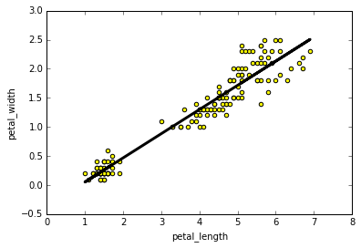
And also plot our data along with the regression line:
1
2
3
4
| import matplotlib.pyplot as plt
axes = iris.plot(x="petal_length", y="petal_width", kind="scatter", color="yellow")
plt.plot(iris["petal_length"], results.predict(), color='black', linewidth=3)
plt.show()
|
|
|---|
| python linear regression - statsmodels |
Method 3: scikit-learn
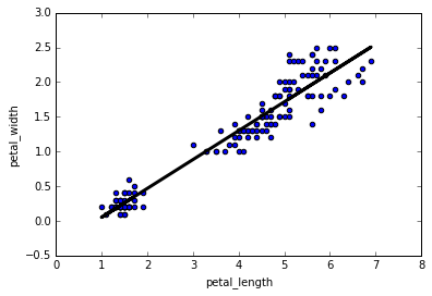
This final examples use scikit-learn, a python library which implements a range of machine learning tools for data analysis - including linear regression. scikit-learn (sklearn) is built around numpy arrays rather than pandas dataframes. To get around this we can reshape the ‘.values’ outputs from the dataframe columns. Once the data is reshaped, the regression is done in much the same way to my other examples.
1
2
3
4
5
6
7
8
9
10
11
12
13
14
15
| from sklearn import datasets, linear_model
import pandas as pd
import matplotlib.pyplot as plt
# Reshape dataframe values for sklearn
fit_data = iris[["petal_length", "petal_width"]].values
x_data = fit_data[:,0].reshape(-1,1)
y_data = fit_data[:,1].reshape(-1,1)
# Create linear regression object
regr = linear_model.LinearRegression()
# once the data is reshaped, running the fit is simple
regr.fit(x_data, y_data)
# we can then plot the data and out fit
axes = iris.plot(x="petal_length", y="petal_width", kind="scatter")
plt.plot(x_data, regr.predict(x_data), color='black', linewidth=3)
plt.show()
|
|
|---|
| python linear regression - sklearn |